Abstract
Hyperparameter estimation is critical for fitting response surface models like Kriging, based on Gaussian Kernels. Traditional estimation methods using the maximum marginal likelihood (MML) function often face optimization difficulties, especially when dealing with noisy or unevenly distributed data. Regularization can alleviate this problem but adds another hyperparameter to identify. A more robust alternative lies in utilizing Bayesian statistics, where each model hyperparameter is estimated through a probability distribution. This approach leverages the likelihood function and priors for each hyperparameter, using the Bayes rule, offering a potentially more resilient method for hyperparameter estimation. The text below elaborates on this process, providing a comprehensive example to illustrate the methodology.
Response surface models based on Gaussian Kernels, such as Kriging, require the estimation of hyperparameters to fit the model to the training data. Commonly, this estimation is made by exploiting the maximum marginal likelihood (MML) function to find the hyperparameter vector \Theta that corresponds to the best likelihood.
However, this is not an easy optimization problem due to the topology of the MML function. Especially for cases, where the data is noisy or unevenly distributed in the parameter space, the optimization might fail, and the resulting response surface model will not fit the data well. While introducing regularization can mitigate this problem, this also adds an additions hyperparameter to the model, which needs to be identified.
An alternative – and more robust – approach to hyperparameter estimation can be based on Bayesian statistics. In this approach each model Hyperparameter is estimated by a probability distribution. The posterior distribution is calculated utilizing the likelihood function and a prior for each hyperparameter, by applying the Bayes rule:
![]()
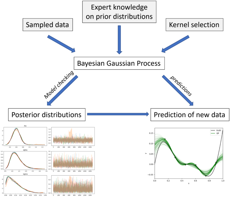
The hyperparameter priors must be chosen by the user and rely heavily on experience, especially if low amounts of training data are available. The posterior distribution is sampled, using an optimized Hamiltonian Monte Carlo (HMC) sampling strategy. Elaborating the resulting sampling-chains insights the convergence of the hyper parameter and thereby allows for some plausibility checks. Two examples are given in the following table. Here, the convergence of the length-scale parameters from a one-dimensional Kriging-model is plotted.

In the “Convergence Failed” case, the estimated hyperparameter distribution does not converge to a stable solution, as it is the case in the “Converged Hyperparameter” case, but rather implies a bi-modal behavior of the modeled process. This can point towards high noise in the input dataset and is accounted by setting the prior for noise modelling to a wider distribution.
The posterior distributions can now be used to predict unknown function-values and give local error estimates for the unknowns. Each hyperparameter is sampled from its posterior distribution N-times, and thereby a probability distribution for each unknown function-value is created and the mean value, as well as the confidence intervals can be extracted. The following graph shows an example, where a noisy 1D function was modeled utilizing the Bayesian Gaussian Process (B-GP) model. The Ground truth is shown by the black curve and the green ones indicate N=1000 samples drawn from the B-GP hyperparameter posterior distributions.

The benefit of that approach becomes apparent when considering the use case of surrogate based optimization, which is demonstrated here with a three-dimensional test function that maps to a scalar value. In practice, this could be three geometry parameters (x1, x2, x3) that influence the drag coefficient (y) of a vehicle.
![]()
The global minimum of this generic process (y = -1) is located at [x1, x2, x3] = [0, -1, 0].
Within the parameter space 32 samples were selected using the Halton sequence. The function was evaluated, artificial random noise (\epsilon) was added to the result and a response surface model was calculated with a MML-based Gaussian Process (ML-GP). As is apparent from the plot below, which compares the exact solution with the predicted solution for 100 test samples (that were not used for model training), the model produced performs excellent for this space filling sampling plan with an R2 score of approximately R2 ~ 0.98.

The picture changes significantly, when additional samples are added based on the expected improvement criterion – a common adaptive sampling strategy for optimization. Local clustering of noisy data leads to model breakdown, even though more information is actually fed into the model. Below the result for the initial 32 Halton samples and 16 additional EI samples is plotted, where the identical optimization strategy fails that worked perfectly fine on the initial dataset.
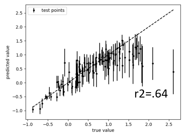
In other words: the tested best practice broke down when data was added – about the opposite of what one wants when adding information to the model.
This is where the superior fitting capability of the Bayesian Gaussian Process (B-GP) becomes obvious. The plots below show the performance of the B-GP-based response surface model for the initial and the final dataset.
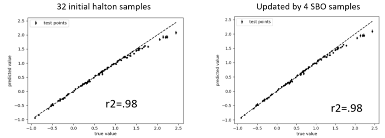
The priors automatically produce a regularization for each new dataset and noise in the data is not learned, thus resulting in a robust response surface modelling that can be trusted in automated processes.